When a Machine Speaks.
Inside the Architecture of a Real-Time Voice AI Agent
On this page
- 1The moment the user speaks
- 2The pipeline at 10,000 feet
- 3How audio gets to your system and back
- 3.1Why this layer exists
- 3.2The browser / app path (WebRTC)
- 3.3The phone path (telephony / PSTN)
- 3.4Why it matters downstream
- 4How computers hear: sound as data
- 4.1What sound physically is, and how a computer listens
- 4.2Turning a wave into numbers: sampling
- 4.3What the waveform hides
- 4.4Putting time back in: the spectrogram
- 4.5Tuning the picture to human ears
- 4.6The whole journey, end to end from the POV of a computer
- 5Getting audio in and out of a real system
- 5.1Sound in slices: frames and streams
- 5.2The bouncer: Voice Activity Detection
- 5.3The return trip: getting sound back out
- 6Speech-to-Text: turning the voice into words
- 6.1Audio in, text out, as it happens
- 6.2Guesses that firm up: partial and final transcripts
- 6.3What actually bites you in production
- 7The LLM: the brain on a stopwatch
- 8Text-to-Speech: turning words back into voice
- 8.1Text in, speech out, as it streams
- 8.2The quality-versus-speed dial
- 8.3What actually bites you in production
- 9The orchestration layer, the part nobody talks about
- 9.1What orchestration actually means
- 9.2Interruption handling (barge-in)
- 9.3End-of-turn detection
- 9.4The latency budget
- 9.5Why frameworks like Pipecat exist
- 10What I left out, and what’s next
- 11Credits & references
The moment the user speaks
A phone rings somewhere, gets picked up, and a voice says “hello?” Another voice answers, asks how it can help, waits, responds to the problem, and the call goes on like any other. Nothing about it feels remarkable. That is exactly the point: one of those voices is not human, and for the few hundred milliseconds between the caller finishing a sentence and the agent starting its reply, it does not feel like a machine at all.
Underneath that one effortless-seeming second, a lot just happened. The caller’s voice had to travel across a network, get sliced into tiny frames, be checked for whether it was even speech, get transcribed into text, get understood by a language model that then decided what to say, have that reply turned back into a human-sounding voice, and have that audio shipped all the way back, all fast enough that the silence never stretched long enough to feel wrong. What feels like a single smooth thing is really six or seven separate systems running a relay race against the clock.
I have spent the last while building one of these in production, and this blog is the map I wish I had when I started, the one that connects the audio, the models, and the glue that holds it all together.
By the end, you’ll understand how a real-time voice agent actually works, end to end, from sound hitting a microphone to the reply coming back, including the orchestration layer that turns out to be the hardest part of all.
The pipeline at 10,000 feet
Before the deep dive into each part, let’s look at the whole pipeline first, so we can see the different pieces and appreciate how many of them have to work together to make a voice AI application real.

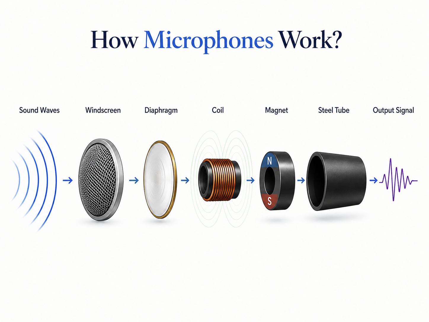
The journey starts with the user’s audio, picked up by the microphone on their device and carried to our server by the transport layer (the connection that moves audio in and out). The sound does not arrive in one big piece; it comes as a stream of tiny chunks called frames. At the entrance sits the VAD, a small model that tracks whether the user is speaking, and its silence signal is what tells the system a turn is over and the LLM should reply. Speech then goes to the STT (speech-to-text), which turns it into a transcript. That text goes to the LLM, which decides what to say. The reply text goes to the TTS (text-to-speech), the opposite of STT, which turns it back into audio. And that audio travels back out over the same transport to be played through the user’s speaker. Getting the audio in and out, that transport step, is itself the subject of the next section.
The key thing to notice is that this is a cascade: each step feeds the next, in order. That simple fact has two consequences that shape everything later in this post. First, the delays add up. Every step takes a little time, and the user doesn’t feel each one separately; they feel the total wait before the bot replies. Second, mistakes carry forward. If the STT mishears a word, the LLM never finds out; it just answers the wrong question, because no later step can fix an error made earlier in the chain.
But here’s what this neat diagram hides. Looking at these tidy boxes and arrows, it’s easy to assume the hard part is building good STT, LLM, and TTS components. It’s not. Those are largely solved pieces you can get from a provider. The hard part is making them work together in real time: handling interruptions, knowing when a person has finished talking, and keeping the whole thing fast. That job belongs to the orchestration layer, the band drawn across the top of the diagram, and it’s the part that most people leave out. It’s where the real difficulty of voice AI lives.
How audio gets to your system and back
Why this layer exists
Before going inside the pipeline, it’s worth pausing on something, how does the user’s voice actually get to the system in the first place, and how does the reply get back? That’s what this section covers. There are mainly two ways a user reaches a voice AI bot: directly through a browser using WebRTC, or through an ordinary phone call. Both are covered below.
The browser / app path (WebRTC)
When the user talks to the bot through a browser or a native app, here’s what happens to their voice on the way in.
The microphone produces raw audio as a stream of numbers, called PCM PCM quality is defined by two independent numbers: sample rate (frequency range) and bit depth (dynamic range). 16-bit PCM gives 65,536 amplitude levels and ~96dB of dynamic range. CD audio is 44.1kHz/16-bit PCM — voice pipelines typically use 16kHz/16-bit, which is enough for speech but cuts the music range. (Pulse Code Modulation), which is just the sound wave sampled thousands of times a second with no compression. Exactly how that sampling turns sound into numbers is the subject of the next section; for now, just picture a long list of numbers describing the sound wave.
Raw PCM is bulky, so before it goes anywhere the browser encodes it into Opus Opus is actually two codecs fused: SILK (Skype's speech codec) handles low-bitrate voice, CELT (a music-quality codec) takes over at higher bitrates — it switches automatically based on content. Range: 6kbps to 510kbps. Standardised by the IETF in 2012 and made the mandatory codec for WebRTC in 2013. , an audio codec built specifically for real-time voice that shrinks the data to a fraction of its size while keeping the quality the human ear cares about. That compressed audio travels over the internet as small real-time packets using WebRTC WebRTC is a full stack, not just a transport: it handles codec negotiation (SDP), NAT traversal (ICE/STUN/TURN), and end-to-end encryption (DTLS-SRTP) automatically. Originally developed by GIPS and On2, acquired by Google, and open-sourced in 2011. The browser's getUserMedia() API sits on top of it. , the browser standard for live audio and video.
One detail matters here: WebRTC sends over UDP, not TCP TCP's specific problem for audio is head-of-line blocking: one lost packet stalls delivery of all subsequent packets until the retransmission arrives. At 20ms frames this stall is immediately audible. WebRTC transmits audio as SRTP (Secure RTP) over UDP — adding encryption without adding TCP's retransmission logic. . With live audio it’s better to drop an occasional packet than to freeze the whole stream waiting for a lost one to be resent, because a late packet is useless once the moment has passed. Speed wins over perfect delivery.
The voice AI server receives these packets, decodes the Opus back into raw PCM, and hands that stream to the pipeline. None of this has to be built from scratch; providers like Daily and LiveKit run the WebRTC infrastructure so you can stay focused on the pipeline.
On the way back out, the reverse happens: the TTS audio is encoded, travels over the same WebRTC connection, and is decoded and played through the user’s speakers.
This browser path is the higher-quality option, carrying 16kHz audio (16,000 samples per second) at low latency, and it is what most people picture when they imagine a modern voice assistant.
The phone path (telephony / PSTN)
Now let us come to the talk of the town, or perhaps the talk of the world. The phone is still how most people make calls, and it runs on the telephone network, which is far older than the internet our browser path was built on.
This is the lower-quality route, but don’t underestimate it: there’s no web or app involved and the user simply dials a number. In most production deployments, particularly contact-center and enterprise use cases, the phone channel is where the bulk of real-world voice AI traffic runs today.
When the user speaks, their phone’s microphone picks up the sound and digitizes it, but this time the audio travels over the telephone network, the PSTN PSTN uses circuit switching: a dedicated 64kbps DS0 channel is reserved end-to-end for the full duration of a call, even during silence. This is why calls were expensive — you were holding a physical circuit open. SIP/VoIP replaces this with packet switching that only consumes bandwidth when audio is actually being sent. (Public Switched Telephone Network), not the internet. It is carried over old circuit-switched infrastructure built for telephony decades ago.
To move across that older network, the audio is encoded as µ-law µ-law (G.711) uses companding — non-linear quantisation that allocates more amplitude levels at quiet volumes, where human hearing is most sensitive. Encodes at 8-bit/sample, 8kHz = 64kbps. Europe uses the nearly identical A-law variant (G.711 A-law). Both standards date to the 1960s and are still the lingua franca of the phone network. (pronounced “mu-law”), an old telephony codec running at 8kHz. That is half the sample rate of the 16kHz browser path, so meaningfully less of the original sound is captured in the first place.
The voice AI server does not speak the telephone network’s language, so something has to bridge the two worlds. That is the job of a telephony provider like Twilio, or a tool like Jambonz: it answers and handles the incoming phone call, then bridges that audio onto a WebSocket connection to the voice AI server (a persistent two-way link), streaming the data in a format the application can actually read. From there it joins the same pipeline as the browser path.
There’s one more step worth being honest about. Because the rest of the pipeline expects 16kHz, the incoming 8kHz audio is upsampled to 16kHz, for example using Pipecat. But this matters: resampling changes the container, not the contents. Stretching 8kHz up to 16kHz doesn’t recover the detail the phone network discarded at capture; it only interpolates between the samples already present. The audio now fits the pipeline’s expected format, but the information lost on the way in stays lost.
On the way back out, the reverse happens: the TTS audio is encoded back to µ-law, handed to the provider, and carried across the phone network to the user’s earpiece.
The honest consequence of all this is quality. The phone path hands the STT model 8kHz audio that has already thrown away much of the original signal, which measurably lowers transcription accuracy compared to the browser path, and nothing at the application level can fix it because the network imposes it. This is the real reason phone-based agents mishear more often than browser-based ones.
Why it matters downstream
The two paths look like a networking detail, but they quietly set the terms for everything that follows. The transport layer decides the format and sample rate of the audio that lands in the pipeline, and every stage after it, starting with the STT model, simply inherits whatever arrived. The channel is usually not a choice; the user’s device decides it, so a robust voice AI pipeline has to handle whatever shows up rather than assume clean 16kHz audio. Frameworks like Pipecat help here by providing ready-made transport components for both paths, so the same pipeline can serve a browser call and a phone call without being rebuilt.
 and the phone path (telephony). Both converge into one internal PCM format before the pipeline sees them.")
The terms “sample rate” and “16kHz versus 8kHz” have come up several times now without a real explanation of what that number is or why it decides how much a model can hear. That is exactly what the next section covers: how raw sound becomes the numbers these models actually work with.
How computers hear: sound as data
This section is the bridge to understanding how the models in the voice AI pipeline actually process sound, so it’s worth getting right before going further. How a computer captures sound as data, stores it, and transforms that stored data into something an ML model can work with is a fascinating topic in its own right, and everything in the model sections ahead rests on it.
What sound physically is, and how a computer listens
So what is sound, really? When anything makes a sound, a voice, a guitar string, a speaker, the object vibrates, and that vibration pushes the surrounding air into tiny travelling waves of pressure. Those pressure waves reach your ear, your eardrum moves in step with them, and your brain decodes that motion into what you experience as sound.
Your ears and brain do this effortlessly. To make a computer do the same, the processing is the part we build later, but what plays the role of the ear? The microphone. Think of a seismograph, the instrument that records earthquakes by tracing a line up and down on paper as the ground trembles. A microphone works on the same principle: it has a part that vibrates in response to the changing air pressure, and a tiny processor measures how far it moves, the amplitude, at each instant, and records that as a number. A short run of these numbers, the slice the pipeline works with at a time, is called a frame, and the full sequence is just a long array of numbers, much like a vector or 1D tensor from ML.

Turning a wave into numbers: sampling
We now have sound arriving as the microphone’s continuous movement. The problem is storing it. Sound is continuous: at every instant the air pressure has some value, with infinitely many instants in between, smooth and unbroken. A computer cannot store something infinite. The way around it is exactly what the microphone does, measure the wave’s height at regular, fixed instants and record each as a number. Picture a graph with time on the x-axis and height on the y-axis: at each fixed interval you place a dot at the wave’s current height. Look at all the dots over time and they trace out the shape of the continuous wave, while staying discrete enough for a computer to store and process. That trick is called sampling.
The sample rate is how many of those snapshots are taken per second, measured in hertz (Hz), which just means “per second.” 16,000 Hz (16kHz) means 16,000 measurements a second; 8kHz means 8,000.
Like video, more frames per second means a smoother, more faithful capture. Audio is the same: more samples per second captures the wave in finer detail. A 5-second clip is 80,000 numbers at 16kHz, but only 40,000 at 8kHz, half as many snapshots of the same wave.
The sample rate also sets a hard ceiling on what can be captured, and the rule is exact:
where is the sample rate and is the highest frequency that can be faithfully represented.
This is the Nyquist limit Without a low-pass anti-aliasing filter before sampling, frequencies above the Nyquist limit don't disappear — they fold back into the audible range as phantom tones (aliasing). Real ADCs always include this filter. CD audio uses 44.1kHz rather than the theoretically sufficient 40kHz specifically to give the filter room to roll off without cutting frequencies the ear can still hear. . The intuition is that you need at least two samples per cycle to capture a wave, one for the peak and one for the trough, so anything vibrating faster than half the sample rate cannot be pinned down and is lost. This is the precise reason the phone path is worse: 16kHz captures up to 8kHz, covering the frequencies that matter most for understanding speech, while 8kHz phone audio caps at 4kHz and loses everything above it, including the high-frequency energy in consonants like “s”, “f”, and “sh”, which is exactly the muffled quality you hear on a call.
One thing the textbooks rarely mention: in a real pipeline, the sample rate isn’t something you pick cleanly, it’s something you fight to keep consistent. Different components and providers expect different rates, and a silent mismatch (audio captured at one rate but read by a model expecting another) doesn’t throw an error; it just quietly wrecks transcription. The failure mode is silent and maddening: audio captured at 8kHz but handed to a component expecting 16kHz doesn’t throw an error — the component reads the samples at the wrong rate, making speech sound slurred and slow to the STT, and accuracy collapses with no obvious cause. A one-line format assertion at the pipeline boundary saves hours of debugging.

What the waveform hides
So we have the sound as a list of sampled numbers. The graph just used to picture sampling is exactly what is called a waveform, the shape most people associate with sound. It plots amplitude over time, which is why this is the time-domain view, time runs along the x-axis.
But this view has a problem. It represents the sound faithfully and can play it back perfectly, yet loudness over time is not what tells one speech sound from another. Take the word “hello”: two of its sounds can have similar-looking waveforms, because what separates them is hidden in the shape, not visible in the up-and-down.
So if loudness over time is not what distinguishes speech sounds, what is? The answer is frequencies. A frequency is just how fast the air pressure wave vibrates, measured in cycles per second, which is what a hertz is, and we hear it as pitch: fast vibrations sound high, slow vibrations sound low. Any sound, however complex, is a mixture of many simple frequencies layered together, a low rumble is a low frequency, a high hiss is a high frequency, and a real sound like a voice is dozens of frequencies present at once, at different strengths.
The best way to feel this is a pianist. When three keys are pressed at once, they leave the piano as a single combined pressure wave, but when it reaches your ear, your brain separates that one wave back into the three distinct notes. That act, going from “the combined wave over time” to “which individual frequencies are present and how strong each is,” is the shift from the time domain to the frequency domain.
So there are two ways to look at the exact same sound. The time domain (the waveform) shows how loud it is at each moment. The frequency domain (the spectrum) shows which frequencies are present and how strong each one is. These are two views of the same data, neither adding nor removing anything, and the mathematical method that breaks a wave into its component frequencies is called the Fourier transform Speech processing uses the Short-Time Fourier Transform (STFT), not the full FT: the signal is split into short overlapping windows (typically 25ms, stepping every 10ms) and the FFT is applied to each window independently. The FFT (Cooley-Tukey algorithm, 1965) makes each window O(n log n) instead of O(n²) — fast enough to run in real time on a CPU. . (A natural question: if they hold the same information, why convert at all? Because what is hidden in one view is laid bare in the other.)
Why this matters for speech: each vowel and consonant has a characteristic pattern of frequencies. The “e” in “hello” concentrates its energy at certain frequencies, the “o” at different ones. The frequency view reveals exactly the fingerprint the waveform hid, which is why models want the frequency view, not the raw wave.
One honest note before going further. Understanding this representation matters, because it’s how you reason about what a model can and cannot hear, why an 8kHz phone call limits accuracy, why background noise sits where it does in the picture. But in a cascaded production pipeline you rarely build any of it by hand. The STT and TTS providers own this layer inside their own black boxes; you hand them audio and get back text, or hand them text and get back audio. The mental model is essential; writing the librosa code for it in production is not.
")
")
Putting time back in: the spectrogram
The frequency view gives the recipe of a sound, but it hides one thing: it gives the recipe of one chunk treated as a whole. It tells you which frequencies are present, but not when each occurred. It is a frozen snapshot.
For a single steady tone that is fine, the recipe never changes. But speech is the opposite of steady. Saying “hello,” the recipe changes constantly: “h” has one recipe, “e” another, “ll” another, “o” another, all within a few hundred milliseconds, and that movement is what carries the meaning. Take the spectrum of the whole word at once and you get a smeared average, losing the order entirely.
Notice the bind: the waveform had time but hid the frequencies; the spectrum reveals the frequencies but loses time. Each has exactly half of what speech needs, which is both.
The spectrogram is the fix, and the idea is almost obvious once the problem is clear. Instead of one spectrum for the whole sound, chop the audio into many tiny slices, each a few milliseconds long, short enough that the sound is roughly steady within it, take the frequency recipe of each slice on its own, and lay the slices side by side in time order, left to right. Time is rebuilt: reading left to right walks forward through the sound, and at each position you see the frequency recipe at that instant. The result is an image, time across the bottom, frequency up the side, brightness showing how strong each frequency is at each moment.
That image is the spectrogram, frequency, time, and strength fused into one picture. The mental image that nails it is sheet music: it shows which notes are played and exactly when, read left to right. A spectrogram is sheet music for any sound. For speech, the vowels appear as bright horizontal bands at their characteristic frequencies, and you can watch them slide as the speaker moves from sound to sound.
")
Tuning the picture to human ears
The spectrogram is excellent, but it has one mismatch with the thing that ultimately matters, human hearing, and fixing it is the whole reason for the mel version.
On a normal spectrogram the frequency axis is linear, evenly spaced: the distance from 100Hz to 200Hz is the same as from 5,000Hz to 5,100Hz. But human ears do not work that way. The jump from 100Hz to 200Hz is enormous, a full octave, an obviously different pitch; the same 100Hz jump from 5,000Hz to 5,100Hz is barely noticeable. Our sensitivity is dense at the low end and stretched thin at the high end, scaling roughly logarithmically. So a linear spectrogram spends its detail in the wrong places, lavishing resolution on high-frequency differences we mostly ignore and under-representing the low-frequency region where the meaningful content of speech actually lives.
The mel scale fixes this by re-spacing the frequency axis to match how humans perceive pitch, more rows packed into the low frequencies where the ear is sensitive, fewer covering the high frequencies where it is not. (“Mel” comes from “melody.”) A mel spectrogram is the same frequency-over-time picture, warped onto this human-hearing scale, usually compressed to something like 40 or 80 mel bands instead of hundreds of linear bins. The effect is a representation tuned to perception rather than raw physics, concentrating detail exactly where it helps distinguish speech sounds.
And that is the destination, the payoff for the whole chain. STT and TTS models take the mel spectrogram as their input and output. An STT model “listens” by reading a mel spectrogram; a TTS model “speaks” by producing one, which a separate model called a vocoder WaveNet (DeepMind, 2016) was the neural vocoder breakthrough but ran at ~0.001× real-time — usable only for pre-generated audio. HiFi-GAN (2020) changed this: it generates audio ~100× faster than real-time on a GPU and ~10× on CPU, making streaming TTS practical. Most production TTS providers use HiFi-GAN or a derivative under the hood. converts back into an actual waveform.
So when a later section says “the model transcribes the audio,” what is physically happening is that the audio became a mel spectrogram and the model read that picture. The mel spectrogram is the interface between sound and the neural networks, which is exactly why it is worth understanding before the model sections.
This is also where the earlier point about sample rate stops being abstract. Because an 8kHz phone call has thrown away everything above 4kHz before the mel spectrogram is ever computed, the upper rows of that picture, the detail the model would use to tell similar sounds apart, simply are not there. In practice this showed up as noticeably worse transcription on phone audio than on browser audio in the same system, and no amount of downstream processing brought it back, because the model can only read what survived capture.
")
The whole journey, end to end from the POV of a computer
Trace the whole journey once. Sound leaves the speaker as a continuous pressure wave; the microphone samples it into a finite array of numbers, and the sample rate decides how much of the original survives, which is why phone audio is muffled. Plotting those numbers over time gives the waveform, which stores the sound faithfully but hides what distinguishes one speech sound from another. That distinguishing information lives in the frequencies, so the waveform is converted into a spectrum; the spectrum is sliced and stacked over time into a spectrogram; and the spectrogram is warped onto the mel scale to match human hearing. The result, the mel spectrogram, is what the models actually read and write. Everything from here on, the STT that hears and the TTS that speaks, operates on this representation, so with it in hand, the rest of the pipeline is ready to make sense.
Getting audio in and out of a real system
We know how the user’s audio reaches the system and what that audio actually is. Between the raw stream arriving and the STT model receiving clean input sits a layer of real engineering, the plumbing most ML-focused explanations skip. This section covers that layer, and the matching work on the way back out.
Sound in slices: frames and streams
Picture talking to someone who does not react at all until you completely stop, then pauses to register that you stopped, then starts processing, then finally replies. It would feel robotic. Since the whole goal is to behave the way a human would, the audio cannot be handled as one big recording processed after the user finishes.
Instead it arrives in small bits, usually 20ms each, and each bit is a frame. The number of samples in a frame is simply:
where is the sample rate in Hz and is the frame duration in seconds.
For a 16kHz WebRTC stream with a 20ms frame: samples. Our telephony path at 8kHz gives only samples per frame — around 320 bytes, half the data, one more reason phone audio is harder downstream. The system processes frames as they arrive, not after the fact, which is what lets the bot react in real time. Individual frames are classified as they come, but the decisions built on top of them, like detecting that speech has started or stopped, look at a short rolling window of recent frames rather than any single one, so a momentary blip doesn’t flip the system’s state.
One deliberate choice happens right at the entrance. Frames do not arrive identically from every transport: some carriers deliver compressed µ-law at 8kHz, others deliver linear PCM, and sample rates vary too. Rather than make every downstream component aware of where the call came from, everything is normalized to one internal PCM format at the entry boundary, so by the time audio reaches STT it is always plain linear PCM regardless of what came in over the wire. This is the practical face of the sample-rate point from the last section: get this boundary wrong and every stage after it silently suffers.
The bouncer: Voice Activity Detection
Say you are using Siri, or the voice mode in an LLM chat app. How would it feel if the system reacted to every cough and bit of room hum? Frustrating. What stops it is the VAD, the Voice Activity Detection model.
VAD Silero VAD — the most widely used open-source VAD with Pipecat — is a ~1MB ONNX model that runs in under 1ms per 30ms frame. Traditional VAD relied on energy thresholds and zero-crossing rates: fast, but easily fooled by background noise. WebRTC also ships its own three-mode VAD (quality / low-bitrate / very-aggressive) used internally by its echo canceller. is a small binary classifier that runs on each frame and predicts the probability that the frame contains human speech rather than silence or noise. That per-frame probability is smoothed over a short window, so the system only declares speech started or stopped once the signal is consistent. It’s deliberately small, cheap, and fast, giving its prediction in around a millisecond or less per frame, which is what lets it run on every frame without slowing anything down. A well-known example is the Silero VAD model, commonly used with Pipecat.1
Getting VAD to behave is a real hassle. Set the confidence threshold too high and quiet speech or trailing words get missed; too low and every small sound counts as speech. Finding that goldilocks zone takes a lot of testing on real audio, and the right values shift with the microphone, the channel, and the background. This unglamorous tuning is a surprisingly large part of making an agent feel reliable. When the STT provider owns VAD, you lose the ability to interrupt early. The barge-in signal can only fire after the STT has committed a final transcript — meaning the bot may keep talking for an extra 200–400ms after the user starts speaking. Running your own VAD keeps the interrupt path fast and independent of the STT’s turn-detection timing.
When you do run your own, it does two jobs. It gates the stream, so only likely-speech frames go onward, saving the cost of activating STT and everything after it on silence. And it acts as an event source: the moments speech starts and stops are exactly the signals the turn-taking logic needs, and that stop signal is the acoustic half of the end-of-turn detection in the orchestration section. That’s why VAD belongs with the turn-taking logic rather than buried in the raw transport, its real output isn’t just filtered audio but the speech events that drive the conversation.
The return trip: getting sound back out
It’s tempting to think the hard part is done once the pipeline is handed clean audio. But the output has to be delivered just as carefully, and most explanations skip it.
The TTS produces its audio in chunks, and how those are handled depends on the mode. In a streaming setup the transport paces the audio out itself on a timed loop, so it plays smoothly without extra buffering on our side. In a non-streaming setup the chunks are accumulated into a small buffer and released once they reach a sensible size. Either way the goal is the same: if the words arrived in uneven little bursts with gaps between them it would sound stuttering, so the system delivers one continuous stream even though it was generated in pieces.
The non-obvious part shows up on interruption. When the user barges in, stopping the TTS isn’t enough, and clearing our own side isn’t enough either, because most of the audio the user is still hearing is no longer on our side at all: it’s already been shipped over the wire to the telephony provider, which is buffering and playing it. So a barge-in flush is really three actions: clear the local buffer, reset the transport’s pacing, and send an explicit kill-audio control message to the provider telling it to drop what it has already queued. This is the real mechanism behind the interruption handling from the orchestration section, and it’s something you only discover once you’ve shipped a phone agent, the “stop talking” command has to travel all the way out to the carrier, not just stop a local generator.
Speech-to-Text: turning the voice into words
Audio in, text out, as it happens
The voice AI bot has its own real-time transcriber, and it’s called STT.
STT, speech to text, is the ML model that takes in the audio and produces a text transcript. From the last section you already know what it’s really doing under the hood: the audio becomes a mel spectrogram, and the model reads that picture and turns it into words. How that model is actually built and trained, the architectures behind it, is a topic big enough for its own post; here the focus is on how STT behaves as a component in a live pipeline.
There are two ways the transcription can happen: batch and streaming. Batch is when you have the whole audio in hand and run the model once to get the transcript, which is fine for something like transcribing a recording, but useless for a live voice bot, because we can’t wait for the user to finish speaking before we even start. So production voice agents use streaming: a live connection stays open, the audio frames from the last section are fed in as they arrive, and the transcript comes back continuously instead of all at once at the end.
Guesses that firm up: partial and final transcripts
Now that streaming is the way real-time agents work, there are two kinds of transcript it gives back: interim (partial) transcripts and final transcripts.
As the audio streams in, the STT keeps emitting its best guess so far, and that guess updates as more audio arrives. Say someone is asking to book a table; the partials might evolve like “I”, “I want”, “I wand”, “I want to”, “I want to book”, correcting themselves as more context comes in, until the model is confident the segment is done and commits a final: “I want to book a table.” Partials are unstable by nature, they are the model’s guess from incomplete audio, so more audio can change them, which is exactly why we never act on a partial. They are useful for things like live captions or giving the system a head start, but not for decisions.
The final is what we actually act on and send to the LLM for the next steps. Here’s the part worth getting right, because it’s the seam between this section and the orchestration layer later: the STT produces these finals on its own, as it detects natural pauses and endpoints in the audio. We don’t tell it “the turn is over” to make it emit a final. It’s the other way around, the orchestration layer takes the STT’s finals together with the silence signal from VAD (and sometimes a dedicated turn-detection model) to decide that the user’s turn is actually over. So the final transcript is one of the inputs to that turn decision, not the result of it.
What actually bites you in production
Everything so far has been how STT is supposed to work. This part is about what happens once real users start calling, because that’s where the surprises live, and a few of them are the kind of thing you only learn the hard way.
Start with the strangest one: your own latency dashboard can quietly lie to you. The obvious number to watch is how long the STT takes to return its first byte, and most frameworks report it for you. But some STT models manage their own turn-taking, and for those the “first byte” they report is actually measured from when the user started talking to when their turn ended, so it’s really measuring how long the user spoke, not how long the model took to process. Plotted as latency, a perfectly healthy system looks broken. We only caught it because the numbers on real calls made no sense, and we had to build a separate metric to recover the STT’s true processing time. The lesson is worth carrying through the rest of this section: an obvious dashboard number can be an artifact of the architecture rather than a real measurement, and you only find out by staring at production traffic.
The rest are smaller, but they are the settings that quietly decide whether the agent feels responsive or broken. Three are worth knowing:
- Endpointing has to stay in sync with VAD. STT providers expose an endpointing setting, how long a pause counts as the end of a chunk, and the defaults can be aggressively short, on the order of milliseconds, which finalises mid-sentence on a phone call where people pause naturally. You raise it to a few hundred milliseconds, but the real catch is that it has to agree with the VAD silence window from the last section. If the two disagree about how long a pause means “done,” your turn detection ends up fighting itself.
- Interim results are a latency lever, not just captions. Keeping partials switched on is not only for live feedback. Turn them off and the system has to wait for the whole utterance to finalise before it sees anything, adding a few hundred milliseconds of dead time to every turn. So the partials we said you should never act on still earn their keep by shaving real latency off the conversation.
- Warm the connection before the call. Pure plumbing nobody mentions: opening a fresh STT connection on the first word can cost a couple of seconds, which is unacceptable on the very first turn. So the connection is opened and kept alive in advance, ready for audio the instant the user speaks.
The LLM: the brain on a stopwatch
This is the brain of the operation, the part of the voice bot that decides what to actually say. You can get the transcription perfect and the speech crystal clear, but if the content of the reply is bad, none of the rest matters.
The first thing that matters here isn’t quality, it’s latency, because the LLM is the single slowest step between the user finishing and the bot replying. In a chat app, latency is forgiving: you can show a buffering icon and the user happily waits. In a voice call, that same wait is dead silence on the line, which feels broken and awkward. This changes how you pick a model. In a chat app you reach for the biggest, most capable model you can. In voice you often do the opposite: deliberately choose a smaller, faster model and cap how much it’s allowed to say, because every extra token is extra time the user spends waiting in silence.
This is also why streaming the output is non-negotiable here. In a chat app you can afford to wait for the LLM to finish its full autoregressive generation before showing anything. In a voice bot you can’t, because if you wait for the whole reply before speaking, the silence stretches long enough that the user thinks the call has dropped. So the LLM streams its tokens out, and the TTS starts speaking the first sentence while the model is still generating the rest.
The format of the output matters too. On a screen, markdown, bullet points, and headings are helpful. Spoken aloud, they’re nonsense: the TTS can’t read a bullet point, and “option one colon” is not how a person talks. So the LLM has to be prompted to produce plain, speakable sentences, the way someone would actually say them out loud, not the way they would format a document.
Finally, tool calling, the thing that turns a plain LLM into an agent that can actually do things: book the table, check the order status, start the process running. It sounds like a perfect fit for voice, and it is, but it’s harder to pull off in a live call than in a chat app. A tool call adds a round trip right in the middle of the latency budget: the model decides to call the tool, the tool runs, the result comes back, and only then can the model produce its spoken reply. In the dead-silence economy of a phone call, that gap is brutal, which is why voice agents often say something like “let me check that for you” to fill the wait before the tool runs. Keeping that brain working, and controlling it, all inside a live call, is its own kind of hard.
Text-to-Speech: turning words back into voice
Text in, speech out, as it streams
So now it is time for the actual voice of the bot. Whether it sounds calm or excited, soft or booming, or like Amitabh Bachchan himself, all the glory goes to the TTS.
TTS is the mirror image of STT: where STT took audio and gave back text, TTS takes the text from the LLM and gives back audio. And from the audio section you already know what’s happening inside: the model produces a mel spectrogram, and a vocoder turns that into the actual waveform, which is sent to the user’s device and played through the speakers. How the model is built and trained is a topic for its own post; here the focus is on how TTS behaves as a component in a live pipeline.
The key behavior is streaming, and it pairs with the LLM from the last section. The LLM streams its text out token by token, and the TTS starts speaking the first sentence while the rest is still being generated. That head start matters, the most perfect, natural-sounding voice in the world counts for nothing if it arrives late and the user is already sitting in silence. In a live call, fast and good-enough beats perfect and late.
The quality-versus-speed dial
Every TTS selection is a trade-off. The richest, most natural-sounding voices tend to carry higher processing times, and in a live call, latency is always a constraint. The model you can actually use in production is the one that sounds good enough and starts fast enough, not just the one with the most impressive demo reel.
The reassuring part is that once you’ve picked a fast-enough voice, TTS is largely a solved part of the latency problem: the first audio comes back quickly and consistently, turn after turn. The time in a voice agent doesn’t really go here. It goes upstream, in deciding the user has finished and in the model thinking up its reply, which is exactly where the next section’s latency budget will point.
What actually bites you in production
So with the voice streaming and the quality dial set, here is what actually goes wrong once real conversations start.
Like STT, you almost never train your own TTS. You call a provider, ElevenLabs, Cartesia, and others,2 and they differ less on raw quality these days and more on how they behave in a live setting: how fast the first audio chunk comes back, how cleanly they stream, and how natural they sound on your particular kind of text. The right choice is the one that holds up on real traffic, not the one with the most impressive demo reel.
And the behavior can be genuinely counterintuitive. You can stream text into a TTS in different granularities, sentence by sentence or token by token, and you’d assume that feeding it smaller, more frequent chunks always gets the first audio out faster. It doesn’t, and which way wins depends entirely on the provider’s engine. With one provider, switching to token-level streaming saved a few hundred milliseconds and we shipped it. With another, the exact same change made things slower, because that engine waits to accumulate a bit of text before it starts synthesizing, so flooding it with tiny fragments worked against it. Same setting, opposite result, and the only way to know was to measure each one.
The thing that separates a good-sounding agent from a robotic one is prosody, the rhythm, emphasis, and intonation of speech. A human raises their pitch at the end of a question, pauses at a comma, and stresses the word that matters. Modern TTS does a lot of this on its own, but it takes its cues from the text it’s given, which is exactly why the speakable-output point from the LLM section matters so much: feed it clean, well-punctuated, plain sentences and it sounds human; feed it markdown or a wall of text with no punctuation and the prosody falls apart.
That connection to the text is sharpest with the awkward bits: phone numbers, dates, currency, and acronyms are all landmines. Should “2024” be spoken as “two thousand twenty four” or “twenty twenty four”? Is “Dr.” the title or the road? Does “$5.50” come out as “five dollars fifty” or “dollar five point five zero”? Providers do some of this normalization on their end, but the most reliable fix is to handle it one layer up, in the LLM prompt, telling the model to write numbers as words and keep its output plainly speakable. The cleanest place to solve a speech problem turns out to be the layer that actually understands the context, not the one just synthesizing audio.
This gets harder the moment more than one language is involved. In a market like India, a single sentence often mixes English words into a Hindi or Tamil utterance, and the pronunciation has to switch mid-sentence without mangling either language. In practice the honest approach is to pick a language-capable voice per call and lean on the provider’s own engine to handle the within-sentence switching, rather than trying to tag every word’s language yourself. Code-switching, proper nouns, and regional pronunciation are real, unglamorous problems that most Western voice-AI writing never touches, and they’re a large part of what it actually takes to sound natural to real users.
And that closes the tour of the components. The transport, the audio representation, the STT, the LLM, and the TTS are all in place now. But a collection of good components isn’t yet a conversation. Making them work together, in real time, without stepping on each other, is a different problem altogether, and it’s where the real difficulty of voice AI lives.
The orchestration layer, the part nobody talks about
What orchestration actually means
Back in the overview, when we saw the pipeline from 10,000 feet, we saw the individual components, the STT, the LLM, the TTS, each doing their job, connected by arrows that make it all look clean and self-sufficient. It’s tempting to assume the intelligence of each model is enough; that each component somehow knows the status of the others and when it should wait or act. But arrows on a diagram don’t run themselves, and that’s exactly the problem the orchestration layer exists to solve.
If you’re familiar with agents in the AI/ML space, the concept will feel familiar. The agent framework, essentially software code like LangGraph or CrewAI, is the orchestrator that makes the LLM capable of executing tools and interacting with the world, rather than just generating text. In the case of voice, this dependency goes to the next level because the pipeline isn’t just passing text between components, it’s passing audio, transcripts, token streams, and synthesized speech, all in real time, with no tolerance for a dropped handoff.
The data starts as raw audio and by the time it exits the pipeline as spoken words, it has been converted across multiple formats at multiple stages. Everything has to flow and hand off seamlessly to make the user feel like they’re talking to a real human.
This is where an orchestration framework like Pipecat comes into the picture. It takes the output of one component and delivers it to the next in the right format at the right moment, while handling silence detection, turn detection, and latency management. A reliable, real-time voice AI agent is only possible because of this orchestration layer. The clearest way to understand what that coordination looks like in practice is to look at what happens when a user interrupts the agent mid-sentence.
Interruption handling (barge-in)
Picture a frustrated customer on a support call. The agent starts its scripted reply, but that’s not what they need, so they cut in: just give me a fast solution or I’m escalating.
Zoom in on that moment. You interrupted while the other person was speaking. They immediately stopped talking, switched to listening, held on to everything that had been said so far, and then responded to your new demand. It’s actually a very complex thing your brain does, coordinating multiple senses in real time, and it feels effortless only because biology has optimized it over millions of years. In a voice AI pipeline we’re trying to replicate that same behavior across multiple separate components, WebSocket connections, hardware limits, and latency, and all of it has to be managed by the orchestration layer to feel natural.
In a production voice AI system, when the user interrupts the bot mid-sentence, three things have to happen at almost the same time.
First, the TTS playback has to stop, and this is harder than it sounds. By the time the user interrupts, a chunk of the agent’s reply has usually already been generated and shipped out ahead of what the user has actually heard, and on a phone call most of that audio is no longer even on our side; it’s sitting in the telephony provider’s buffer being played out. So stopping the model isn’t enough. As we saw in the return-trip section, the buffered audio has to be flushed everywhere it lives, which on a phone call means sending an explicit kill-audio message all the way out to the carrier. Miss any of that and the agent keeps talking for a noticeable moment after the user has started speaking.
Second, the in-flight LLM call has to be handled. Implementations differ here. The simpler approach cancels the generation entirely and starts fresh with the new user input. The more sophisticated approach pauses generation, prepends the new user input to the existing context, and lets the LLM respond with full awareness of what it had already started saying. Both are valid; the right choice depends on how much conversational continuity your use case demands. Either way, the LLM must be given the context that the user barged in so it doesn’t continue as if its interrupted answer was delivered.
Third, the STT, which until now was mostly ignoring background noise, has to switch back to actively listening and push the user’s new speech forward through the pipeline as a fresh turn. If this switch is slow, the first word or two of what the user says gets missed.
The point is that this is an absolute coordination game between components. If STT starts listening before TTS has fully stopped, the agent’s own voice can be picked up and transcribed as user input. If the LLM lags, a stale response can arrive even after the user has moved on. The orchestration layer is the driver that keeps all of this in sync.
And here’s the genuinely hard part, the one that makes you appreciate your own biology. Short sounds like “hmm”, “ok”, or a cough are not real interruptions, but if the system treats them as one, the agent stops constantly and the conversation falls apart. Humans make this judgment without thinking. One way to approximate it in production is to use an LLM as a judge to decide whether an incoming sound is a real interruption or just noise. That’s only one mitigation, and it’s far from a solved problem — distinguishing a real barge-in from a backchannel “mhm” is still an open corner of voice AI.

End-of-turn detection
Watch a great speaker, Steve Jobs, Richard Feynman, anyone who thinks in public, and you’ll notice they pause between thoughts, sometimes for a beat that feels long. Yet as a listener you don’t jump in. You somehow know they’re not done. How does that happen, and how do we replicate it in software?
When you examine what your brain is doing, it turns out you’re combining two signals. First, you detect the silence itself. Second, you take into account the context of the conversation and what the person said just before the silence. Together, those two signals tell you whether their turn is actually over or whether they’re still going.
A voice AI pipeline does the same thing with two components. VAD detects acoustic silence and how long it has lasted. A separate turn-detection model, such as Smart Turn from Pipecat, listens to the audio of what was just said and judges whether the utterance sounds complete.3 It does this by analyzing the raw waveform directly, not the transcript, which is exactly what lets it catch fillers like “um” and “hmm” that transcription models silently drop. The result: “what are your business” sounds unfinished; “what are your business hours” does not. Some turn detectors work off the transcript text instead; Smart Turn’s waveform-first approach is the key design difference. The main tuning knob is the silence threshold, and good systems make it adaptive. A system might use a 200ms threshold when the utterance sounds complete, and extend that to 400ms or more when it sounds mid-sentence. That difference of a few hundred milliseconds is what separates a system that feels responsive from one that constantly cuts people off.
Getting this wrong is costly in both directions, and you’ve felt both as a user. End the turn too eagerly and the agent cuts you off, which feels rude. Wait too long and it feels sluggish, leaving you wondering if it even heard you. No threshold gets it right for everyone: fast talkers, slow talkers, non-native speakers, and anyone reading out a phone number or email all break the simple rules. The silence-plus-semantics heuristic is what most production systems actually run on today, and tuning it carefully for your specific user base is one of the less glamorous but most impactful things you can do for conversation quality.
The latency budget
There’s a number that matters more than almost any other in a voice agent: the gap between the moment you stop talking and the moment the bot starts. Too long, and the user wonders if it even heard them. Long enough, and they hang up.
The key thing about latency is that it behaves like a budget. The stages run sequentially, so their delays add up:
For the conversation to feel human, needs to stay under roughly 800ms; past about 1.5 seconds the user notices the lag and starts to disengage. Here’s where the milliseconds go in a typical cascaded setup, with industry-consensus ranges next to what I measured in my own system.
| Stage | What happens | Typical range | My system (warm avg) |
|---|---|---|---|
| End-of-turn detection | Deciding the user has finished speaking | 150 to 300 ms | folded into the silence-wait, see below |
| Speech-to-text | Finalising the transcript | 100 to 300 ms | part of the ~110 ms pipeline + STT-final |
| LLM time-to-first-token | The model producing the first chunk of its reply | 300 to 800 ms | ~670 ms (72%) |
| Text-to-speech first audio | First reply chunk turned into the first audio frame | 75 to 200 ms | ~151 ms (16%) |
| Network and pipeline overhead | Transport hops, encoding, buffering, glue | 50 to 150 ms | included above |
| Total (end-of-turn to first audio) | ~700 to 1500 ms | ~900 ms |
The ranges are wide because the numbers swing with model choice, region, and prompt size, so read them as the shape of the budget, not fixed costs. My ~900ms total sits right in the realistic production band, where most deployed agents land.
Look at where the time actually goes. The LLM, not the speech models, takes the biggest slice of the budget, which surprises people who assume STT or TTS is the bottleneck. The reason is that an LLM is autoregressive Generates one token at a time, each conditioned on the ones before it — so the reply can only be produced sequentially, not all at once. : it generates its reply one token at a time, each token conditioned on the last, and before it can emit even the first token it has to process the entire input context, the system prompt plus the whole conversation history.
That’s why this number grows as your prompt grows, while streaming STT and TTS stay roughly flat.
But that 900ms hides something important. It measures from the moment the system decides you’ve stopped talking, not from the moment you actually stopped. The silence-wait before that decision happens off the clock.
In my setup that wait is about 500ms, which pushes the latency the user actually feels to roughly 1.4 seconds, not 900ms. So if you only instrument the pipeline from end-of-turn onward, your dashboards say you’re fast while your users sit through a real lag. The number that matters is measured from the user’s last word to the agent’s first word, and it’s always bigger than your component metrics suggest.
This led to a result that surprised me. I compared two setups: one with a dedicated turn-detection stack (Silero VAD plus SmartTurn), and one letting the STT provider drive end-of-turn directly, no turn models in the path. On paper the smarter stack should win.
It didn’t, at least not on perceived speed. The raw pipeline total was a tie, but the turn-detection stack carried a higher silence-wait floor (around 500ms versus 350ms), making it about 130ms slower from the caller’s point of view, and less consistent turn to turn.
To be clear, this was a small test, a few dozen turns, not a benchmark. The lesson isn’t that SmartTurn is worse; it’s that the smarter component doesn’t automatically win once you measure latency the way the user feels it. Measure perceived latency on your own traffic and let the numbers decide.

Why frameworks like Pipecat exist
Step back and look at what the last three sections had in common. Interruption handling, turn detection, latency management, none of it is specific to any one product. Every voice agent needs all of it, no matter which STT, LLM, or TTS providers it happens to use. It’s the same coordination problem solved over and over again.
That’s exactly the gap a framework fills. Pipecat is the open-source framework that handles this coordination layer for you, so you’re not rebuilding cancellation, buffering, and turn logic from scratch on every project.4 When the user barges in, for example, it’s Pipecat’s pipeline that propagates the interrupt and cancels the in-flight stages, the messy choreography we walked through in the interruption section.
from pipecat.pipeline.pipeline import Pipelinefrom pipecat.services.deepgram import DeepgramSTTServicefrom pipecat.services.openai import OpenAILLMServicefrom pipecat.services.cartesia import CartesiaTTSService
pipeline = Pipeline([    transport.input(),   # audio frames in (WebRTC or telephony)    stt,                 # speech -> text (streaming, emits finals)    llm,                 # text -> reply tokens (streaming)    tts,                 # tokens -> audio chunks    transport.output(),  # audio frames back out])
A minimal Pipecat pipeline wiring Deepgram STT → OpenAI LLM → Cartesia TTS. In a real deployment each service is initialised with API keys and model config before being passed in; the structure here shows the shape of the chain, not production-ready code.
The trade-off is real, though. A framework gives you all of this for free, but you give up some control over exactly how each piece behaves, which starts to matter the moment you need something the framework didn’t anticipate.
Under the hood this coordination is built out of a few core abstractions, frames, frame processors, and context aggregators, that turn the messy choreography of the last few sections into something composable. That machinery is a deep topic in its own right, but the takeaway here is simpler: the orchestration layer is what quietly turns a collection of fast individual models into something that feels like a single, responsive voice.
What I left out, and what’s next
If you’ve made it all the way here, you’ve gone deeper into voice AI than almost anyone who hasn’t built one, and that’s worth something. Thank you for staying.
A quick honest note on what this post is not. It’s one architecture, the cascaded STT-LLM-TTS pipeline, and there’s a whole other approach worth its own post: speech-to-speech models, where a single model hears and replies directly, with no pipeline of separate parts at all. I also deliberately stopped at the edge of several deep topics. The internals of the STT and TTS models, how they’re actually built and trained. The internals of an orchestration framework like Pipecat, its frames and processors and aggregators. And the whole craft of latency optimization, which is where a lot of my own time has gone: moving from fresh HTTP requests to persistent connections, warming every network hop before the call so the first turn isn’t the slowest, and the optimizations that sounded smart but did nothing measurable. Each of those deserves its own post rather than a paragraph here.
This was the post I wish I had when I started working in this space, a single place that connects the audio, the models, and the glue into one picture. The next one will go a level deeper, into the STT model itself, how it actually works and how it’s trained.
You can find me on LinkedIn, and you can subscribe to get the next post straight to your inbox. Until then, take care.
lvnb now signing off.
Credits & references
The pipeline overview, barge-in sequence, latency-budget waterfall, and sampling figures are my own (Excalidraw / matplotlib). The microphone cross-section and seismograph illustrations are original, generated for this post. The latency numbers are measurements from my own production system, not borrowed benchmarks.
- Audio representation figures (waveform, spectrum, spectrogram, mel spectrogram) — Hugging Face Audio Course, Unit 1.
- Concepts and pipeline framing are informed by the Pipecat documentation and the sources footnoted throughout. All prose is my own.
Footnotes
-
Silero VAD — github.com/snakers4/silero-vad ↩
-
Providers worth knowing: ElevenLabs, Cartesia, Deepgram Aura, and OpenAI. ↩
-
Smart Turn, Pipecat’s open-source turn-detection model — docs.pipecat.ai/server/utilities/smart-turn/smart-turn-overview ↩
-
Pipecat pipeline guide — docs.pipecat.ai/guides/learn/pipeline ↩